WIKI de Bertrand VANDEPORTAELE

Table des matières

The Homography model
Compute an image given an original image and the homography between the 2 image planes
Estimation of Homography from 2D points correspondances using the DLT algorithm
- Checking the obtained results
- Normalization of the data for least squares fitting
Uncertainty propagation

The Homography model

Compute an image given an original image and the homography between the 2 image planes

 function imout=CalculeImageHomographie(H,imout,hautout,largout,imin,hautin,largin)
%fonction imout=CalculeImageHomographie(H,imout,hautout,largout,imin,hautin,largin)
%@Bertrand VANDEPORTAELE
%La fonction calcule l'image imout à partir de l'image imin
%H= homographie entre les 2 images tel que imout= H*imin
%imout= image de sortie, elle est aussi en entrée, car on peut la modifier
%hautout,largout= dimensions de l'image de sortie
%imin= image d'entrée
%hautin,largin= dimensions de l'image d'entrée
%%%%%%%%%%%%%%%%%%%%%%%%%%%%%%%%%%%%%%%%%%%%%%%%%%%%%%%%%%%%%%%%%%%%%%%%%%%
for y=1:hautout
    for x=1:largout
        p2=H*[x,y,1]'; %transformation homographique inverse
        ud=round(p2(1)/p2(3));
        vd=round(p2(2)/p2(3));
        ud;
        vd;
        if vd>0 & ud>0 & vd<=hautin & ud<=largin
            %ca tombe dans l'image
            val=imin(vd,ud);
            imout(y,x)=val; %on attribue la couleur du pixel concerné
        else
            %ca tombe hors de l'image datamatrix, on laisse la valeur du
            %fond
            %eventuellement, on aurait pu faire:
%            imout(y,x)=255; %on attribue la couleur blanche
        end
    end
end

Estimation of Homography from 2D points correspondances using the DLT algorithm

compute2DHomographyUsingDLT.m

function [ H] = compute2DHomographyUsingDLT( p1,p2)
%B. Vandeportaele
%compute the Homography H using the DLT Algorithm for 4 2D points 
%correspondences such as : p2=H.p1
u11=p1(1,1);u12=p1(1,2);
u13=p1(1,3);u14=p1(1,4);
v11=p1(2,1);v12=p1(2,2);
v13=p1(2,3);v14=p1(2,4);
 
u21=p2(1,1);u22=p2(1,2);
u23=p2(1,3);u24=p2(1,4);
v21=p2(2,1);v22=p2(2,2);
v23=p2(2,3);v24=p2(2,4);
 
A=[ -u11, -v11, -1,    0,    0,  0, u11*u21, u21*v11;
    0,    0,  0, -u11, -v11, -1, u11*v21, v21*v11;
    -u12, -v12, -1,    0,    0,  0, u12*u22, u22*v12;
    0,    0,  0, -u12, -v12, -1, u12*v22, v22*v12;
    -u13, -v13, -1,    0,    0,  0, u13*u23, u23*v13;
    0,    0,  0, -u13, -v13, -1, u13*v23, v23*v13;
    -u14, -v14, -1,    0,    0,  0, u14*u24, u24*v14;
    0,    0,  0, -u14, -v14, -1, u14*v24, v24*v14];
B =[ -u21; -v21; -u22; -v22; -u23; -v23; -u24; -v24];
%solve A*Hv=B
Hv=inv(A)*B;
%reconstruct the homography matrix from the vector solution
H=[Hv(1:3)';Hv(4:6)';Hv(7:8)',1];
end

Checking the obtained results

check2DHomography.m

function [ err] = check2DHomography(H, p1,p2 )
%B. Vandeportaele
%compute the error in R2 (after deshomogeneisation) for every points 
%contained in p1 and p2 matrices considering the homography H
%err= p2 -deshomogenieisation(H.p1)
err=[];
for i=1:size(p1,2)
    u11=p1(1,i);
    v11=p1(2,i);
    wuv21p=H*[u11;v11;1];
    err(1,i)=p2(1,i)-(wuv21p(1)/wuv21p(3));
    err(2,i)=p2(2,i)-(wuv21p(2)/wuv21p(3));
end
end

Normalization of the data for least squares fitting

normalizeForH.m

function [ p2, s,tx,ty] = normalizeForH( p1 )
%B. Vandeportaele
%normalization of the data for homography estimation. Scale s and 
%translation (tx,ty) is computed to obtain a distribution of point with 0 
%mean and sqrt(2) std dev.
%as explained in Geometry in Computer Vision (2ed,OUP,2003)(T)(672s)
% Data Normalization p107 & p180
 
%transform p1 points to p2 such that p2 points are centered around 0:0 and mean distance to 0:0 is sqrt(2)
 
%eventually see page 128 for the case where some points in p1 are very far away from the origin
%it would require a complete homography instead of just a scaling and
%translation, as it involve dealing with p1 in projective space P2
 
%in page 109, it is explained that non isotropic scaling is not necessary.
 
 
%average distance
m=mean(p1,2)';
 
%p1-[m(1)*ones(1,size(p1,2));    m(2)*ones(1,size(p1,2))]
%translation to bring the centroid at 0:0
dist=[];
for i=1:size(p1,2)
    pc(1:2,i)=p1(:,i)-m'; %centered points
    dist(i)=norm(pc(1:2,i),2);
end
meandist=mean(dist)
s=sqrt(2)/meandist;
 
for i=1:size(p1,2)
    p2(1:2,i)=s*pc(:,i); %scaled and centered points
end
tx=-s*m(1);
ty=-s*m(2);
 
end

Uncertainty propagation

jaco.m

%B. Vandeportaele
%script to achieve symbolic computation of the jacobian
% du2/dHij
% dv2/dHij
% Hij being the coefficients of the homography such as
% w.u2       u1
% w.v2 = H . v1
%   w.        1
clear all
 
param=1
 
h11=sym('h11','real');h12=sym('h12','real');h13=sym('h13','real');
h21=sym('h21','real');h22=sym('h22','real');h23=sym('h23','real');
h31=sym('h31','real');h32=sym('h32','real');h33=sym('h33','real');
%possibly use 2 parameterization for the homography, h33 may be set to 1
if param==0
    H=[h11 h12 h13; h21 h22 h23;h31 h32 h33]
else
    H=[h11 h12 h13; h21 h22 h23;h31 h32 1]
end
 
u1=sym('u1','real');
v1=sym('v1','real');
 
P1=[u1;v1;1];
%apply the homography
P2=H*P1
%deshomogeneization
u2=P2(1,:)/P2(3,:)
v2=P2(2,:)/P2(3,:)
%compute the jacobians
if param==0
    J=jacobian ([u2, v2], [h11, h12, h13, h21, h22, h23, h31, h32, h33])
else
    J=jacobian ([u2, v2], [h11, h12, h13, h21, h22, h23, h31, h32])
end

Conclusion for param=1: $J= \left(\begin{array}{cccccccc} \frac{\mathrm{u1}}{\mathrm{h31}\, \mathrm{u1} + \mathrm{h32}\, \mathrm{v1} + 1} & \frac{\mathrm{v1}}{\mathrm{h31}\, \mathrm{u1} + \mathrm{h32}\, \mathrm{v1} + 1} & \frac{1}{\mathrm{h31}\, \mathrm{u1} + \mathrm{h32}\, \mathrm{v1} + 1} & 0 & 0 & 0 & -\frac{\mathrm{u1}\, \left(\mathrm{h13} + \mathrm{h11}\, \mathrm{u1} + \mathrm{h12}\, \mathrm{v1}\right)}left_mathrm_h31_mathrm_u1_mathrm_h32_mathrm_v1_1_right_2_-_frac_mathrm_v1_left_mathrm_h13_mathrm_h11_mathrm_u1_mathrm_h12_mathrm_v1_right_left_mathrm_h31_mathrm_u1_mathrm_h32_mathrm_v1_1_right_2_0_0_0_frac_mathrm_u1{\mathrm{h31}\, \mathrm{u1} + \mathrm{h32}\, \mathrm{v1} + 1} & \frac{\mathrm{v1}}{\mathrm{h31}\, \mathrm{u1} + \mathrm{h32}\, \mathrm{v1} + 1} & \frac{1}{\mathrm{h31}\, \mathrm{u1} + \mathrm{h32}\, \mathrm{v1} + 1} & -\frac{\mathrm{u1}\, \left(\mathrm{h23} + \mathrm{h21}\, \mathrm{u1} + \mathrm{h22}\, \mathrm{v1}\right)}{{\left(\mathrm{h31}\, \mathrm{u1} + \mathrm{h32}\, \mathrm{v1} + 1\right)}^2} & -\frac{\mathrm{v1}\, \left(\mathrm{h23} + \mathrm{h21}\, \mathrm{u1} + \mathrm{h22}\, \mathrm{v1}\right)}{{\left(\mathrm{h31}\, \mathrm{u1} + \mathrm{h32}\, \mathrm{v1} + 1\right)}^2} \end{array}\right)$ <file matlab usejaco3.m> %B. Vandeportaele %script to illustrate uncertainty propagation for homography (projective %transformation) clear all %%%%%%%%%%%%%%%%%%%%%%%%%%%%%%%%%%%%%%%%%%%%%%%%%%%%%%%%%%%%%%%%%%%%%%%%%%% %define 4 set of 2 2D points correspondances such as % w.u21 u11 % w.v21 = H . v11 % w. 1 % position u11,v11 in plane 1 is supposed to be perfectly known u11=0;v11=0; u12=1;v12=0; u13=0;v13=1; u14=1;v14=1; %%%%%%%%%%%%%%%%%%%%%%%%%%%%%%%%%%%%%%%%%%%%%%%%%%%%%%%%%%%%%%%%%%%%%%%%%%% %position u21,v21 in plane 2 is associated with a covariance matrix u21=10;v21=10; u22=150;v22=40; u23=30;v23=130; u24=190;v24=210; %%%%%%%%%%%%%%%%%%%%%%%%%%%%%%%%%%%%%%%%%%%%%%%%%%%%%%%%%%%%%%%%%%%%%%%%%%% %covariance for the point's positions in plane 2. std dev are square roots %of the diagonal values %default value: Cp=1*eye(8) %change the value as needed if uncertainty are not the same for all the %points if 1 Cp(1,1)=3; Cp(2,2)=5; Cp(3,3)=10; Cp(4,4)=25; Cp(5,5)=50; Cp(6,6)=1; Cp(7,7)=0.1; Cp(8,8)=0.1; end %%%%%%%%%%%%%%%%%%%%%%%%%%%%%%%%%%%%%%%%%%%%%%%%%%%%%%%%%%%%%%%%%%%%%%%%%%% %store coordinates in matrices p1=[u11,u12,u13,u14;v11,v12,v13,v14] p2=[u21,u22,u23,u24;v21,v22,v23,v24] %%%%%%%%%%%%%%%%%%%%%%%%%%%%%%%%%%%%%%%%%%%%%%%%%%%%%%%%%%%%%%%%%%%%%%%%%%% %DLT Algorithm: [ H] = compute2DHomographyUsingDLT( p1,p2) %%%%%%%%%%%%%%%%%%%%%%%%%%%%%%%%%%%%%%%%%%%%%%%%%%%%%%%%%%%%%%%%%%%%%%%%%%% %check computed H, should be 0 [ err] = check2DHomography(H, p1,p2 ) %%%%%%%%%%%%%%%%%%%%%%%%%%%%%%%%%%%%%%%%%%%%%%%%%%%%%%%%%%%%%%%%%%%%%%%%%%% h11=H(1,1);h12=H(1,2);h13=H(1,3); h21=H(2,1);h22=H(2,2);h23=H(2,3); h31=H(3,1);h32=H(3,2);h33=H(3,3); %compute J numerically then invert the 8x8 matrix to obtain Ji J =[]; % computed in jaco.m: J=jacobian ([u2, v2], [h11, h12, h13, h21, h22, h23, h31, h32]) for i=1:4 u1=p1(1,i);v1=p1(2,i); J=[J; u1/(h31*u1 + h32*v1 + 1), v1/(h31*u1 + h32*v1 + 1), 1/(h31*u1 + h32*v1 + 1), 0, 0, 0, -(u1*(h13 + h11*u1 + h12*v1))/(h31*u1 + h32*v1 + 1)^2, -(v1*(h13 + h11*u1 + h12*v1))/(h31*u1 + h32*v1 + 1)^2; 0, 0, 0, u1/(h31*u1 + h32*v1 + 1), v1/(h31*u1 + h32*v1 + 1), 1/(h31*u1 + h32*v1 + 1), -(u1*(h23 + h21*u1 + h22*v1))/(h31*u1 + h32*v1 + 1)^2, -(v1*(h23 + h21*u1 + h22*v1))/(h31*u1 + h32*v1 + 1)^2]; end J detJ=det(J) %check if detJ is high enough, otherwise it won't be invertible in %practice if detJ<0.01 display 'the system looks ill-conditionned' return; end Ji=inv(J) %%%%%%%%%%%%%%%%%%%%%%%%%%%%%%%%%%%%%%%%%%%%%%%%%%%%%%%%%%%%%%%%%%%%%%%%%%% % In case we want to estimate H from more than 4 correspondances, get from: % http://stackoverflow.com/questions/30737382/getting-covariance-matrix-when-using-levenberg-marquardt-lsqcurvefit-in-matlab % I think I have solved this myself but will post how here if anyone else is having the same trouble. % The covariance matrix can be calculated from the Jacobian by: % C = inv(J'*J)*MSE % Where MSE is mean-square error: % MSE = (R'*R)/(N-p) % Where R = residuals, N = number of observations, p = number of coefficients estimated. % Or MSE can be calculated via iteration. % Hopefully this will help someone else in the future. % If anyone spots error please let me know. Thanks %QUESTION????? in that case what is the inverse of the (non square) jacobian for the inverse homography H^-1 %propagation of thee covariance to the coefficients of H Ch=Ji*Cp*Ji' detCh=det(Ch) %what is the meaning of that value: look at %https://math.stackexchange.com/questions/889425/what-does-determinant-of-covariance-matrix-give %compute the covariance on the coefficients of the 2D points, it should give %the same value than Cp Cp2=J*Ch*J' ErrorCp=Cp-Cp2 %%%%%%%%%%%%%%%%%%%%%%%%%%%%%%%%%%%%%%%%%%%%%%%%%%%%%%%%%%%%%%%%%%%%%%%%%%% %Plot the uncertainty on a grid sampled in plane 1 %%%%%%%%%%%%%%%%%%%%%%%%%%%%%%%%%%%%%%%%%%%%%%%%%%%%%%%%%%%%%%%%%%%%%%%%%%% close all figure hold on axis equal for u15=-2:.25:2; for v15=-2:.25:2; wuv25=H*[u15;v15;1]; u25=wuv25(1)/wuv25(3); v25=wuv25(2)/wuv25(3); Jp=[ u15/(h31*u15 + h32*v15 + 1), v15/(h31*u15 + h32*v15 + 1), 1/(h31*u15 + h32*v15 + 1), 0, 0, 0, -(u15*(h13 + h11*u15 + h12*v15))/(h31*u15 + h32*v15 + 1)^2, -(v15*(h13 + h11*u15 + h12*v15))/(h31*u15 + h32*v15 + 1)^2; 0, 0, 0, u15/(h31*u15 + h32*v15 + 1), v15/(h31*u15 + h32*v15 + 1), 1/(h31*u15 + h32*v15 + 1), -(u15*(h23 + h21*u15 + h22*v15))/(h31*u15 + h32*v15 + 1)^2, -(v15*(h23 + h21*u15 + h22*v15))/(h31*u15 + h32*v15 + 1)^2]; Cp5=Jp*Ch*Jp'; plotcovar(u25,v25,Cp5,'r+','b-'); end end %plot the covariance for the four 2D point correspondances used by DLT for i=1:4 u2=p2(1,i);v2=p2(2,i); Cpi=Cp(1+(i-1)*2:2+(i-1)*2,1+(i-1)*2:2+(i-1)*2); plotcovar(u2,v2,Cpi,'g+','g-'); end %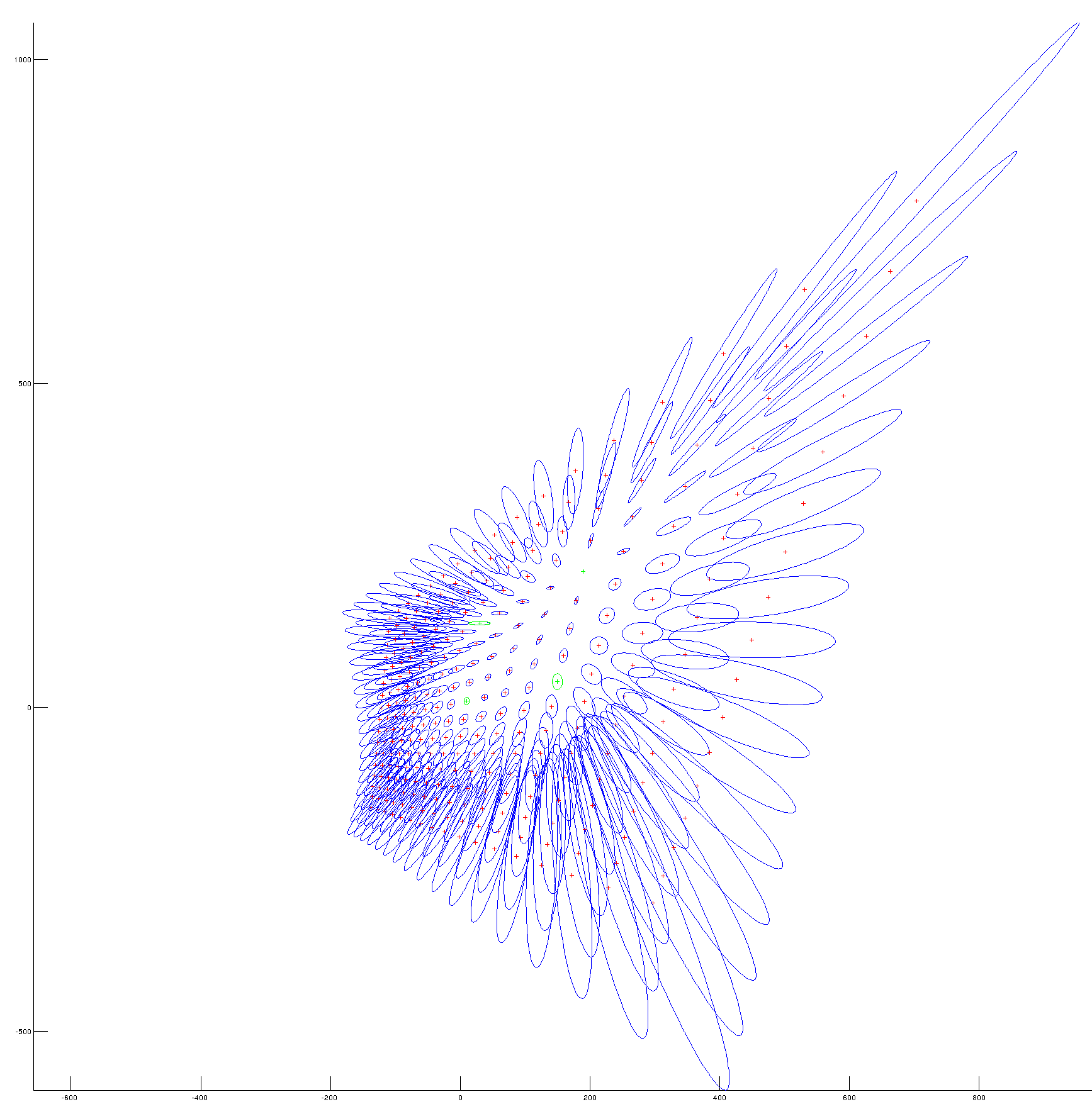en vert, 4 points (et leur incertitude) utilisés pour estimer l'homographie par Direct Linear Transform %en rouge, des points auquel on applique l'homographie calculée (interpolation et extrapolation) %et en bleu l'incertitude de l'homographie estimé propagée à ces points </file> ====Function to plot the covariance==== <file matlab plotcovar.m> function plotcovar(u,v,C,m1,m2) %get from http://www.visiondummy.com/2014/04/draw-error-ellipse-representing-covariance-matrix/ % Get the 95% confidence interval error ellipse chisquare_val = 2.4477; %INFO: pour une covariance=identité, trace un cercle de RAYON chisquare_val %pour une covariance diagonale, les termes de variance sont les carrés des écarts type %l'ellipse tracée un aura ses DEMI-axes de longeur ecart type * chisquare_val %hold on %plotcovar(10,20,[2,4;3,1],'r+','b-'); %plotcovar(10,20,[1,0;0,1],'r+','b-'); plot(u,v,m1) %bvdp, added step to inforce that C is symetric %if this precaution is not taken, this kind of matrix can be provided %C=[0.999999999999951 2.73114864057789e-14;-1.50990331349021e-14 0.999999999999964] %and it will result in complex eigen value, which won't be treatable by the %atan2 function used later... Cm=(C(2,1)+C(1,2))/2; C(2,1)=Cm; C(1,2)=Cm; % Calculate the eigenvectors and eigenvalues covariance =C; [eigenvec, eigenval ] = eig(covariance); [eigenvec, eigenval ] = eig(covariance,'nobalance'); % Get the index of the largest eigenvector [largest_eigenvec_ind_c, r] = find(eigenval == max(max(eigenval))); largest_eigenvec = eigenvec(:, largest_eigenvec_ind_c); % Get the largest eigenvalue largest_eigenval = max(max(eigenval)); % Get the smallest eigenvector and eigenvalue if(largest_eigenvec_ind_c == 1) smallest_eigenval = max(eigenval(:,2)); smallest_eigenvec = eigenvec(:,2); else smallest_eigenval = max(eigenval(:,1)); smallest_eigenvec = eigenvec(1,:); end % Calculate the angle scriptshellbetween the x-axis and the largest eigenvector angle = atan2(largest_eigenvec(2), largest_eigenvec(1)); % This angle is between -pi and pi. % Let's shift it such that the angle is between 0 and 2pi if(angle < 0) angle = angle + 2*pi; end % Get the coordinates of the data mean avg = [u;v]; %mean(data); theta_grid = linspace(0,2*pi); phi = angle; X0=avg(1); Y0=avg(2); a=chisquare_val*sqrt(largest_eigenval); b=chisquare_val*sqrt(smallest_eigenval); % the ellipse in x and y coordinates ellipse_x_r = a*cos( theta_grid ); ellipse_y_r = b*sin( theta_grid ); %Define a rotation matrix R = [ cos(phi) sin(phi); -sin(phi) cos(phi) ]; %let's rotate the ellipse to some angle phi r_ellipse = [ellipse_x_r;ellipse_y_r]' * R; % Draw the error ellipse plot(r_ellipse(:,1) + X0,r_ellipse(:,2) + Y0,m2) %hold on; % Plot the original data %plot(data(:,1), data(:,2), '.'); %mindata = min(min(data)); %maxdata = max(max(data)); %Xlim([mindata-3, maxdata+3]); %Ylim([mindata-3, maxdata+3]); %hold on; % Plot the eigenvectors %quiver(X0, Y0, largest_eigenvec(1)*sqrt(largest_eigenval), largest_eigenvec(2)*sqrt(largest_eigenval), '-m', 'LineWidth',2); %quiver(X0, Y0, smallest_eigenvec(1)*sqrt(smallest_eigenval), smallest_eigenvec(2)*sqrt(smallest_eigenval), '-g', 'LineWidth',2); %hold on; % Set the axis labels %hXLabel = xlabel('x'); %hYLabel = ylabel('y'); </file> ====Results==== {{https://bvdp.inetdoc.net/files/homography/homographyuncertainty.png}} =====Bi-cubic interpolation of Homographies===== <file matlab bilinearInterpolationMulti.m> function val = bilinearInterpolationMulti(x, y, A) %B. Vandeportaele [haut,larg,nbchannels]=size(A); %preallocate the return value val=zeros(nbchannels,1); u=x; v=y; fu= floor(x); fv = floor(y); A1=(fv+1-v)*(fu+1-u); A2=(fv+1-v)*(u-fu); A3=(v-fv)*(fu+1-u); A4=(v-fv)*(u-fu); %if ( (fu>=0) && (fu<larg-2) && (fv>=0) && (fv<haut-2)) if ( (fu>=1) && (fu<larg-1) && (fv>=1) && (fv<haut-1)) %close enough from the boundaries for n=1:nbchannels val(n)= A1*A(fv,fu,n) ... +A2*A(fv,fu+1,n) ... +A3*A(fv+1,fu,n) ... +A4*A(fv+1,fu+1,n); end else %too close from the boundaries, don't interpolate end </file> <file matlab bicubicInterpolationMulti.m> function val = bicubicInterpolationMulti(x, y, data) %B. Vandeportaele %https://en.wikipedia.org/wiki/Bicubic_interpolation %https://fr.wikipedia.org/wiki/Interpolation_bicubique %A is a k.l.m matrix, m being the number of channels nbchannels=size(data,3); %preallocate the return value val=zeros(nbchannels,1); %Control points x0 = floor(x); y0 = floor(y); x_1 = x0-1; x1 = x0+1; x2 = x0+2; y_1 = y0-1; y1 = y0+1; y2 = y0+2; for n=1:nbchannels % Function evaluated at control points f_1_1 = data(y_1,x_1,n); f_10 = data(y0,x_1,n); f_11 = data(y1,x_1,n); f_12 = data(y2,x_1,n); f0_1 = data(y_1,x0,n); f00 = data(y0,x0,n); f01 = data(y1, x0,n); f02 = data(y2, x0,n); f1_1 = data(y_1, x1,n); f10 = data(y0, x1,n); f11 = data(y1, x1,n); f12 = data(y2, x1,n); f2_1 = data(y_1, x2,n); f20 = data(y0, x2,n); f21 = data(y1, x2,n); f22 = data(y2, x2,n); % Derivatives in x evaluated at control points fx0_1 = (f1_1 - f_1_1)/2; fx00 = (f10 - f_10)/2; fx01 = (f11 - f_11)/2; fx02 = (f12 - f_12)/2; fx1_1 = (f2_1 - f0_1)/2; fx10 = (f20 - f00)/2; fx11 = (f21 - f01)/2; fx12 = (f22 - f02)/2; % Derivatives in y evaluated at control points fy00 = (f01 - f0_1)/2; fy10 = (f11 - f1_1)/2; fy01 = (f02 - f00)/2; fy11 = (f12 - f10)/2; % Derivatives in x and y evaluated at control points fxy00 = (fx01 - fx0_1)/2; fxy10 = (fx11 - fx1_1)/2; fxy01 = (fx02 - fx00)/2; fxy11 = (fx12 - fx10)/2; % Interpolation Px=[1,(x-x0),(x-x0)^2,(x-x0)^3]; %don't know why but sometime the generated Px is a column vector Px=reshape(Px,1,4); Py=[1;(y-y0);(y-y0)^2;(y-y0)^3]; A=[ 1 0 0 0; ... Coefficients aij 0 0 1 0; ... -3 3 -2 -1; ... 2 -2 1 1]; F=[ f00 f01 fy00 fy01; ... f10 f11 fy10 fy11; ... fx00 fx01 fxy00 fxy01; ... fx10 fx11 fxy10 fxy11]; val(n)=Px*A*F*A'*Py; end </file> <file matlab saveRawFloat.m> %%%%%%%%%%%%%%%%%%%%%%%%%%%%%%%%%%%%%%%%%%%%%%%%%%%%%%%%%%%%%%%%%%%%%%%%%% % saveRawFloat save a matlab matrix to a binary file for export. % Input : - mat : matrix to export in a binary file. % - nomfichier : file name of the futur binary file. %%%%%%%%%%%%%%%%%%%%%%%%%%%%%%%%%%%%%%%%%%%%%%%%%%%%%%%%%%%%%%%%%%%%%%%%%%% function saveRawFloat(mat, nomfichier) %saveRawFloat(zeros(4), '../tmp/test.raw') % Compute number of values, we want to save nb=1; for i=1:size(size(mat),2) nb=nb*size(mat,i); end % Open the file fid = fopen(nomfichier, 'wb'); % Save the number of elements fwrite(fid, nb, 'uint32'); % il faudra verifier l'endianess... % Transpose matrix to save data line after line. % Data are saved in simple precision floating point numbers 32 bits. fwrite(fid, mat', 'float'); fclose (fid); </file> <file matlab HomographyInterpolation.m> %B. Vandeportaele October 2017 %Cubic spline interpolation in Homography space for deflectometry close all clear all %%%%%%%%%%%%%%%%%%%%%%%%%%%%%%%%%%%%%%%%%%%%%%%%%%%%%%%%%%%%%%%%%%%%%%%%%%% %set the size of the spline control point grid sx=15; sy=10; %how many sampled pixels between 2 control points in each direction for %the generation of the image samplingfactor=100; %%%%%%%%%%%%%%%%%%%%%%%%%%%%%%%%%%%%%%%%%%%%%%%%%%%%%%%%%%%%%%%%%%%%%%%%%%% %choose the type of interpolation for homography coefficients through %function pointer InterpolationFunction=@bicubicInterpolationMulti; %InterpolationFunction=@bilinearInterpolationMulti; %%%%%%%%%%%%%%%%%%%%%%%%%%%%%%%%%%%%%%%%%%%%%%%%%%%%%%%%%%%%%%%%%%%%%%%%%%% HomographyGrid=zeros(sy,sx,9); %identity matrix by default HomographyDefault=reshape(eye(3),9,1); %if the default value has to be set differently %HomographyDefault=reshape([1,0,65; 0,1,0; 0,0,1],9,1); %fill the grid with the default value for y=1:sy for x=1:sx HomographyGrid(y,x,:)=HomographyDefault; end end %perturbate some control points of the spline HomographyGrid(5,4,:)=reshape([1,0,0; 0,1,0; 0,0,0.9],9,1); HomographyGrid(4,4,:)=reshape([1.3,0,0; 0,1.3,0; 0,0,1],9,1); % HomographyGrid(5,4,:)=reshape([1,0,0; 0,1,0; 0,0,0.22],9,1); % HomographyGrid(5,5,:)=reshape([1,0,0; 0,1,0; 0,0,1.3],9,1); % HomographyGrid(6,5,:)=reshape([1,0,0; 0,1,0; 0,0,1.5],9,1); % HomographyGrid(6,4,:)=reshape([1,0,0; 0,1,0; 0,0,0.3],9,1); % HomographyGrid(6,4,:)=reshape([1.2,0,0; 0,0.9,0; 0,0,1],9,1); HomographyGrid(6,5,:)=reshape([1,0,0; 0,1,0; 0,0,1],9,1); HomographyGrid(6,8,:)=reshape([1,0,60; 0,1,-30; 0,0,1],9,1); %%%%%%%%%%%%%%%%%%%%%%%%%%%%%%%%%%%%%%%%%%%%%%%%%%%%%%%%%%%%%%%%%%%%%%%%%%% %interpolate the homography in a small region at low resolution for %visualization purpose %very unefficient code because the size of the destination matrix are not %known at the begining=> reallocation indy=1; for yy=3:0.1:sy-2 indx=1; for xx=3:0.1:sx-2 %val = InterpolationFunction( xx,yy,HomographyGrid); val = feval(InterpolationFunction, xx,yy,HomographyGrid); indx=indx+1; res(indy,indx,1)=xx; res(indy,indx,2)=yy; res(indy,indx,3)=val(9); InterpolatedFunction(indy,indx,:)=val; end indy=indy+1; end %%%%%%%%%%%%%%%%%%%%%%%%%%%%%%%%%%%%%%%%%%%%%%%%%%%%%%%%%%%%%%%%%%%%%%%%%%% figure axis equal plot3(res(:,:,1),res(:,:,2),res(:,:,3),'r+') %%%%%%%%%%%%%%%%%%%%%%%%%%%%%%%%%%%%%%%%%%%%%%%%%%%%%%%%%%%%%%%%%%%%%%%%%%% figure for channel=1:9 subplot(3,3,channel) imagesc(InterpolatedFunction(:,:,channel)) end %%%%%%%%%%%%%%%%%%%%%%%%%%%%%%%%%%%%%%%%%%%%%%%%%%%%%%%%%%%%%%%%%%%%%%%%%%% %compute correspondance map correspondancemapu=zeros(sy*samplingfactor,sx*samplingfactor); correspondancemapv=zeros(sy*samplingfactor,sx*samplingfactor); for yy=2*samplingfactor:sy*samplingfactor-3*samplingfactor for xx=2*samplingfactor:sx*samplingfactor-3*samplingfactor %if xx==1099 % display 'ici' %end H =reshape( InterpolationFunction( xx/samplingfactor,yy/samplingfactor,HomographyGrid),3,3); p2=H*[xx,yy,1]'; %transformation homographique inverse %ud=round(p2(1)/p2(3)); %vd=round(p2(2)/p2(3)); ud=p2(1)/p2(3); vd=p2(2)/p2(3); correspondancemapu(yy,xx)=ud; correspondancemapv(yy,xx)=vd; end end %%%%%%%%%%%%%%%%%%%%%%%%%%%%%%%%%%%%%%%%%%%%%%%%%%%%%%%%%%%%%%%%%%%%%%%%%%% %save to a correspondance map using an openCV compatible format %file saved with .map extension map=[correspondancemapv;correspondancemapu]; imagedirectory='./'; mapname=sprintf('%s/correspondance.map',imagedirectory); saveRawFloat(map, mapname); display('correspondance.map file saved in imagedirectory'); %future use: process the images using python bindings of opencv remap %function: see /media/HD500GO/saveHDDgarossos/menage_ocamcalib/remap %%%%%%%%%%%%%%%%%%%%%%%%%%%%%%%%%%%%%%%%%%%%%%%%%%%%%%%%%%%%%%%%%%%%%%%%%%% %%% Apply the interpolated homography to a synthetic image. %%% it visualizes the equivalent of the control grid but in the source %%% image plane imoutsinu=zeros(sy*samplingfactor,sx*samplingfactor); imoutsinv=zeros(sy*samplingfactor,sx*samplingfactor); imoutsinuv=zeros(sy*samplingfactor,sx*samplingfactor); imoutsinvu=zeros(sy*samplingfactor,sx*samplingfactor); imoutcircle=zeros(sy*samplingfactor,sx*samplingfactor); imoutradial=zeros(sy*samplingfactor,sx*samplingfactor); imoutgrid=zeros(sy*samplingfactor,sx*samplingfactor); for yy=2*samplingfactor:size(imoutsinu,1)-3*samplingfactor for xx=2*samplingfactor:size(imoutsinu,2)-3*samplingfactor ud=correspondancemapu(yy,xx); vd=correspondancemapv(yy,xx); %for a square grid valpix=127*mod(floor(ud/samplingfactor),2) + 127*mod(floor(vd/samplingfactor),2) ; imoutgrid(yy,xx)=valpix; %on attribue la couleur du pixel concerné %for a sinus wave in u direction valpix=uint8(127+127*sin(ud/2.5)); imoutsinu(yy,xx)=valpix; %on attribue la couleur du pixel concerné %for a sinus wave in v direction valpix=uint8(127+127*sin(vd/2.5)); imoutsinv(yy,xx)=valpix; %on attribue la couleur du pixel concerné %for a sinus wave in uv diagonal direction valpix=uint8(127+127*sin((vd+ud)/(2*2.5))); imoutsinuv(yy,xx)=valpix; %on attribue la couleur du pixel concerné %for a sinus wave in vu diagonal direction valpix=uint8(127+127*sin((vd-ud)/(2*2.5))); imoutsinvu(yy,xx)=valpix; %on attribue la couleur du pixel concerné %for a sinus wave in circle direction valpix=uint8(127+127*sin((norm([(ud-750);(vd-500)],2) /2.5))); imoutcircle(yy,xx)=valpix; %on attribue la couleur du pixel concerné %for a sinus wave in radial direction angle=atan2((vd-500),(ud-750))*20; valpix=uint8(127+127*sin(angle)); imoutradial(yy,xx)=valpix; %on attribue la couleur du pixel concerné end end %%%%%%%%%%%%%%%%%%%%%%%%%%%%%%%%%%%%%%%%%%%%%%%%%%%%%%%%%%%%%%%%%%%%%%%%%%% %display images figure subplot(3,1,1); image(imoutgrid); axis equal;colormap(gray(256)); subplot(3,1,2); image(imoutsinu); axis equal;colormap(gray(256)); subplot(3,1,3); image(imoutsinv); axis equal;colormap(gray(256)); %%%%%%%%%%%%%%%%%%%%%%%%%%%%%%%%%%%%%%%%%%%%%%%%%%%%%%%%%%%%%%%%%%%%%%%%%%% %save images imwrite(uint8(imoutgrid),'imoutgrid.png'); 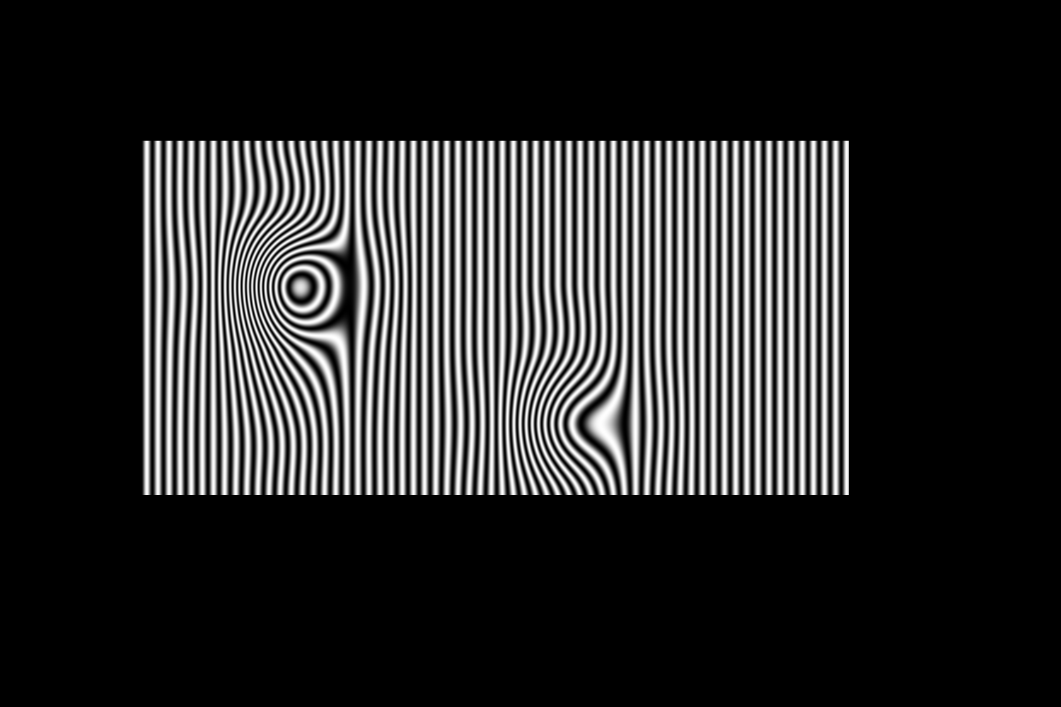imwrite(uint8(imoutsinu),'imoutu.png'); 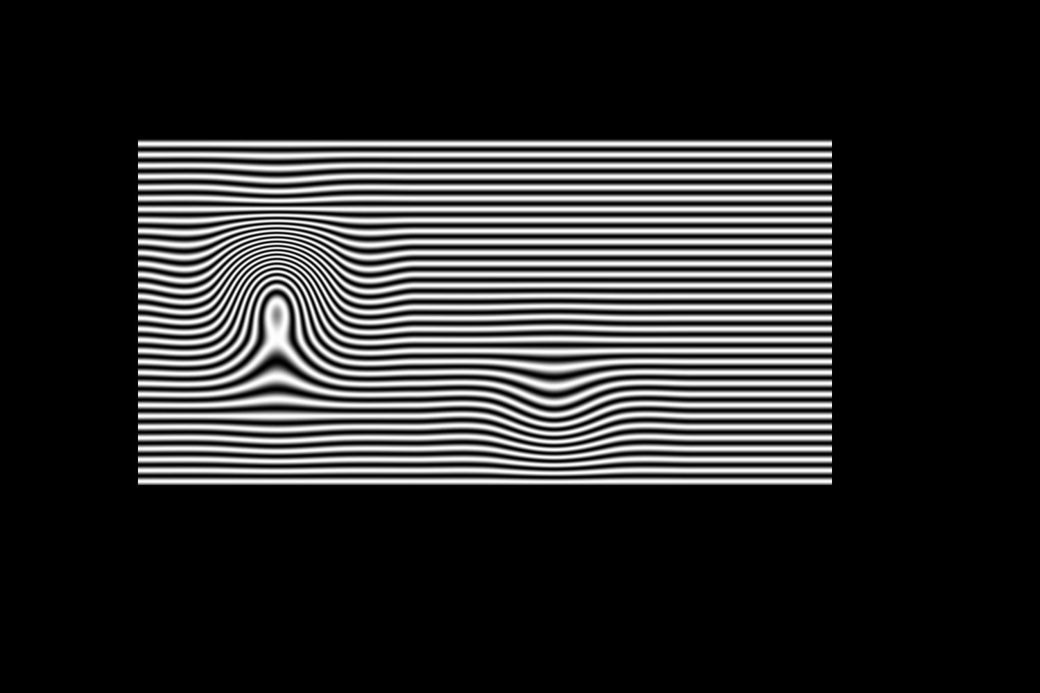imwrite(uint8(imoutsinv),'imoutv.png'); imwrite(uint8(imoutsinuv),'imoutuv.png'); imwrite(uint8(imoutsinvu),'imoutvu.png'); imwrite(uint8(imoutcircle),'imoutcircle.png'); imwrite(uint8(imoutradial),'imoutradial.png'); %%%%%%%%%%%%%%%%%%%%%%%%%%%%%%%%%%%%%%%%%%%%%%%%%%%%%%%%%%%%%%%%%%%%%%%%%%% %generate sequences of images nn=0; for angle=0:2*pi/60:2*pi if angle~=0 nn=nn+1 end for yy=2*samplingfactor:size(imoutsinu,1)-3*samplingfactor for xx=2*samplingfactor:size(imoutsinu,2)-3*samplingfactor ud=correspondancemapu(yy,xx); vd=correspondancemapv(yy,xx); %for a sinus wave in u direction valpix=uint8(127+127*sin(angle+(ud/2.5))); imoutsinu(yy,xx)=valpix; %on attribue la couleur du pixel concerné %for a sinus wave in v direction valpix=uint8(127+127*sin(angle+(vd/2.5))); imoutsinv(yy,xx)=valpix; %on attribue la couleur du pixel concerné end end imgname=sprintf('%s/sinu%02i.png',imagedirectory,nn); imwrite(uint8(imoutsinu),imgname); imgname=sprintf('%s/sinv%02i.png',imagedirectory,nn); imwrite(uint8(imoutsinv),imgname); end %%%%%%%%%%%%%%%%%%%%%%%%%%%%%%%%%%%%%%%%%%%%%%%%%%%%%%%%%%%%%%%%%%%%%%%%%%% %compute the mpg videos... does not work from within matlab, invoke it %through a linux shell %system('avconv -f image2 -i sinu%02d.png -f avi -vcodec mpeg4 -b 4000k -g 300 -bf 2 -y ./videosinu.mpg') %system('avconv -f image2 -i sinv%02d.png -f avi -vcodec mpeg4 -b 4000k -g 300 -bf 2 -y ./videosinv.mpg'); </file> ====Results==== {{https://bvdp.inetdoc.net/files/deflectometry/imoutu.png}} {{https://bvdp.inetdoc.net/files/deflectometry/imoutv.png}} =====Garbage===== $\left(\begin{array}{ccc} {\mathrm{q1}}^2 + {\mathrm{q2}}^2 - {\mathrm{q3}}^2 - {\mathrm{q4}}^2 & 2\, \mathrm{q2}\, \mathrm{q3} - 2\, \mathrm{q1}\, \mathrm{q4} & 2\, \mathrm{q1}\, \mathrm{q3} + 2\, \mathrm{q2}\, \mathrm{q4}\\ 2\, \mathrm{q1}\, \mathrm{q4} + 2\, \mathrm{q2}\, \mathrm{q3} & {\mathrm{q1}}^2 - {\mathrm{q2}}^2 + {\mathrm{q3}}^2 - {\mathrm{q4}}^2 & 2\, \mathrm{q3}\, \mathrm{q4} - 2\, \mathrm{q1}\, \mathrm{q2}\\ 2\, \mathrm{q2}\, \mathrm{q4} - 2\, \mathrm{q1}\, \mathrm{q3} & 2\, \mathrm{q1}\, \mathrm{q2} + 2\, \mathrm{q3}\, \mathrm{q4} & {\mathrm{q1}}^2 - {\mathrm{q2}}^2 - {\mathrm{q3}}^2 + {\mathrm{q4}}^2 \end{array}\right) $ $\left(\begin{array}{ccccccccccc} 2\, \mathrm{q1} & 2\, \mathrm{q2} & - 2\, \mathrm{q3} & - 2\, \mathrm{q4} & -\frac{\mathrm{nx}}{d} & 0 & 0 & -\frac{\mathrm{tx}}{d} & 0 & 0 & \frac{\mathrm{nx}\, \mathrm{tx}}{d^2}\\ - 2\, \mathrm{q4} & 2\, \mathrm{q3} & 2\, \mathrm{q2} & - 2\, \mathrm{q1} & -\frac{\mathrm{ny}}{d} & 0 & 0 & 0 & -\frac{\mathrm{tx}}{d} & 0 & \frac{\mathrm{ny}\, \mathrm{tx}}{d^2}\\ 2\, \mathrm{q3} & 2\, \mathrm{q4} & 2\, \mathrm{q1} & 2\, \mathrm{q2} & -\frac{\mathrm{nz}}{d} & 0 & 0 & 0 & 0 & -\frac{\mathrm{tx}}{d} & \frac{\mathrm{nz}\, \mathrm{tx}}{d^2}\\ 2\, \mathrm{q4} & 2\, \mathrm{q3} & 2\, \mathrm{q2} & 2\, \mathrm{q1} & 0 & -\frac{\mathrm{nx}}{d} & 0 & -\frac{\mathrm{ty}}{d} & 0 & 0 & \frac{\mathrm{nx}\, \mathrm{ty}}{d^2}\\ 2\, \mathrm{q1} & - 2\, \mathrm{q2} & 2\, \mathrm{q3} & - 2\, \mathrm{q4} & 0 & -\frac{\mathrm{ny}}{d} & 0 & 0 & -\frac{\mathrm{ty}}{d} & 0 & \frac{\mathrm{ny}\, \mathrm{ty}}{d^2}\\ - 2\, \mathrm{q2} & - 2\, \mathrm{q1} & 2\, \mathrm{q4} & 2\, \mathrm{q3} & 0 & -\frac{\mathrm{nz}}{d} & 0 & 0 & 0 & -\frac{\mathrm{ty}}{d} & \frac{\mathrm{nz}\, \mathrm{ty}}{d^2}\\ - 2\, \mathrm{q3} & 2\, \mathrm{q4} & - 2\, \mathrm{q1} & 2\, \mathrm{q2} & 0 & 0 & -\frac{\mathrm{nx}}{d} & -\frac{\mathrm{tz}}{d} & 0 & 0 & \frac{\mathrm{nx}\, \mathrm{tz}}{d^2}\\ 2\, \mathrm{q2} & 2\, \mathrm{q1} & 2\, \mathrm{q4} & 2\, \mathrm{q3} & 0 & 0 & -\frac{\mathrm{ny}}{d} & 0 & -\frac{\mathrm{tz}}{d} & 0 & \frac{\mathrm{ny}\, \mathrm{tz}}{d^2}\\ 2\, \mathrm{q1} & - 2\, \mathrm{q2} & - 2\, \mathrm{q3} & 2\, \mathrm{q4} & 0 & 0 & -\frac{\mathrm{nz}}{d} & 0 & 0 & -\frac{\mathrm{tz}}{d} & \frac{\mathrm{nz}\, \mathrm{tz}}{d^2} \end{array}\right)$ $\left(\begin{array}{cccccccc} \frac{u_{1}1}{\mathrm{h31}\, u_{1}1 + \mathrm{h32}\, \mathrm{v11} + 1} & \frac{\mathrm{v11}}{\mathrm{h31}\, u_{1}1 + \mathrm{h32}\, \mathrm{v11} + 1} & \frac{1}{\mathrm{h31}\, u_{1}1 + \mathrm{h32}\, \mathrm{v11} + 1} & 0 & 0 & 0 & -\frac{u_{1}1\, \left(\mathrm{h13} + \mathrm{h11}\, u_{1}1 + \mathrm{h12}\, \mathrm{v11}\right)}{{\left(\mathrm{h31}\, u_{1}1 + \mathrm{h32}\, \mathrm{v11} + 1\right)}^2} & -\frac{\mathrm{v11}\, \left(\mathrm{h13} + \mathrm{h11}\, u_{1}1 + \mathrm{h12}\, \mathrm{v11}\right)}{{\left(\mathrm{h31}\, u_{1}1 + \mathrm{h32}\, \mathrm{v11} + 1\right)}^2}\\ 0 & 0 & 0 & \frac{u_{1}1}{\mathrm{h31}\, u_{1}1 + \mathrm{h32}\, \mathrm{v11} + 1} & \frac{\mathrm{v11}}{\mathrm{h31}\, u_{1}1 + \mathrm{h32}\, \mathrm{v11} + 1} & \frac{1}{\mathrm{h31}\, u_{1}1 + \mathrm{h32}\, \mathrm{v11} + 1} & -\frac{u_{1}1\, \left(\mathrm{h23} + \mathrm{h21}\, u_{1}1 + \mathrm{h22}\, \mathrm{v11}\right)}{{\left(\mathrm{h31}\, u_{1}1 + \mathrm{h32}\, \mathrm{v11} + 1\right)}^2} & -\frac{\mathrm{v11}\, \left(\mathrm{h23} + \mathrm{h21}\, u_{1}1 + \mathrm{h22}\, \mathrm{v11}\right)}{{\left(\mathrm{h31}\, u_{1}1 + \mathrm{h32}\, \mathrm{v11} + 1\right)}^2}\\ \frac{\mathrm{u12}}{\mathrm{h31}\, \mathrm{u12} + \mathrm{h32}\, \mathrm{v12} + 1} & \frac{\mathrm{v12}}{\mathrm{h31}\, \mathrm{u12} + \mathrm{h32}\, \mathrm{v12} + 1} & \frac{1}{\mathrm{h31}\, \mathrm{u12} + \mathrm{h32}\, \mathrm{v12} + 1} & 0 & 0 & 0 & -\frac{\mathrm{u12}\, \left(\mathrm{h13} + \mathrm{h11}\, \mathrm{u12} + \mathrm{h12}\, \mathrm{v12}\right)}{{\left(\mathrm{h31}\, \mathrm{u12} + \mathrm{h32}\, \mathrm{v12} + 1\right)}^2} & -\frac{\mathrm{v12}\, \left(\mathrm{h13} + \mathrm{h11}\, \mathrm{u12} + \mathrm{h12}\, \mathrm{v12}\right)}{{\left(\mathrm{h31}\, \mathrm{u12} + \mathrm{h32}\, \mathrm{v12} + 1\right)}^2}\\ 0 & 0 & 0 & \frac{\mathrm{u12}}{\mathrm{h31}\, \mathrm{u12} + \mathrm{h32}\, \mathrm{v12} + 1} & \frac{\mathrm{v12}}{\mathrm{h31}\, \mathrm{u12} + \mathrm{h32}\, \mathrm{v12} + 1} & \frac{1}{\mathrm{h31}\, \mathrm{u12} + \mathrm{h32}\, \mathrm{v12} + 1} & -\frac{\mathrm{u12}\, \left(\mathrm{h23} + \mathrm{h21}\, \mathrm{u12} + \mathrm{h22}\, \mathrm{v12}\right)}{{\left(\mathrm{h31}\, \mathrm{u12} + \mathrm{h32}\, \mathrm{v12} + 1\right)}^2} & -\frac{\mathrm{v12}\, \left(\mathrm{h23} + \mathrm{h21}\, \mathrm{u12} + \mathrm{h22}\, \mathrm{v12}\right)}{{\left(\mathrm{h31}\, \mathrm{u12} + \mathrm{h32}\, \mathrm{v12} + 1\right)}^2}\\ \frac{\mathrm{u13}}{\mathrm{h31}\, \mathrm{u13} + \mathrm{h32}\, \mathrm{v13} + 1} & \frac{\mathrm{v13}}{\mathrm{h31}\, \mathrm{u13} + \mathrm{h32}\, \mathrm{v13} + 1} & \frac{1}{\mathrm{h31}\, \mathrm{u13} + \mathrm{h32}\, \mathrm{v13} + 1} & 0 & 0 & 0 & -\frac{\mathrm{u13}\, \left(\mathrm{h13} + \mathrm{h11}\, \mathrm{u13} + \mathrm{h12}\, \mathrm{v13}\right)}{{\left(\mathrm{h31}\, \mathrm{u13} + \mathrm{h32}\, \mathrm{v13} + 1\right)}^2} & -\frac{\mathrm{v13}\, \left(\mathrm{h13} + \mathrm{h11}\, \mathrm{u13} + \mathrm{h12}\, \mathrm{v13}\right)}{{\left(\mathrm{h31}\, \mathrm{u13} + \mathrm{h32}\, \mathrm{v13} + 1\right)}^2}\\ 0 & 0 & 0 & \frac{\mathrm{u13}}{\mathrm{h31}\, \mathrm{u13} + \mathrm{h32}\, \mathrm{v13} + 1} & \frac{\mathrm{v13}}{\mathrm{h31}\, \mathrm{u13} + \mathrm{h32}\, \mathrm{v13} + 1} & \frac{1}{\mathrm{h31}\, \mathrm{u13} + \mathrm{h32}\, \mathrm{v13} + 1} & -\frac{\mathrm{u13}\, \left(\mathrm{h23} + \mathrm{h21}\, \mathrm{u13} + \mathrm{h22}\, \mathrm{v13}\right)}{{\left(\mathrm{h31}\, \mathrm{u13} + \mathrm{h32}\, \mathrm{v13} + 1\right)}^2} & -\frac{\mathrm{v13}\, \left(\mathrm{h23} + \mathrm{h21}\, \mathrm{u13} + \mathrm{h22}\, \mathrm{v13}\right)}{{\left(\mathrm{h31}\, \mathrm{u13} + \mathrm{h32}\, \mathrm{v13} + 1\right)}^2}\\ \frac{\mathrm{u14}}{\mathrm{h31}\, \mathrm{u14} + \mathrm{h32}\, \mathrm{v14} + 1} & \frac{\mathrm{v14}}{\mathrm{h31}\, \mathrm{u14} + \mathrm{h32}\, \mathrm{v14} + 1} & \frac{1}{\mathrm{h31}\, \mathrm{u14} + \mathrm{h32}\, \mathrm{v14} + 1} & 0 & 0 & 0 & -\frac{\mathrm{u14}\, \left(\mathrm{h13} + \mathrm{h11}\, \mathrm{u14} + \mathrm{h12}\, \mathrm{v14}\right)}{{\left(\mathrm{h31}\, \mathrm{u14} + \mathrm{h32}\, \mathrm{v14} + 1\right)}^2} & -\frac{\mathrm{v14}\, \left(\mathrm{h13} + \mathrm{h11}\, \mathrm{u14} + \mathrm{h12}\, \mathrm{v14}\right)}{{\left(\mathrm{h31}\, \mathrm{u14} + \mathrm{h32}\, \mathrm{v14} + 1\right)}^2}\\ 0 & 0 & 0 & \frac{\mathrm{u14}}{\mathrm{h31}\, \mathrm{u14} + \mathrm{h32}\, \mathrm{v14} + 1} & \frac{\mathrm{v14}}{\mathrm{h31}\, \mathrm{u14} + \mathrm{h32}\, \mathrm{v14} + 1} & \frac{1}{\mathrm{h31}\, \mathrm{u14} + \mathrm{h32}\, \mathrm{v14} + 1} & -\frac{\mathrm{u14}\, \left(\mathrm{h23} + \mathrm{h21}\, \mathrm{u14} + \mathrm{h22}\, \mathrm{v14}\right)}{{\left(\mathrm{h31}\, \mathrm{u14} + \mathrm{h32}\, \mathrm{v14} + 1\right)}^2} & -\frac{\mathrm{v14}\, \left(\mathrm{h23} + \mathrm{h21}\, \mathrm{u14} + \mathrm{h22}\, \mathrm{v14}\right)}{{\left(\mathrm{h31}\, \mathrm{u14} + \mathrm{h32}\, \mathrm{v14} + 1\right)}^2} \end{array}\right)$ $\left(\begin{array}{c} \frac{\mathrm{fx}\, x + \mathrm{pu}\, z}{z} - \frac{\mathrm{fx}\, x - \mathrm{bp} + \mathrm{pu}\, z}{z}\\ 0 \end{array}\right)$ =====BSPLINES===== $\left(\begin{array}{ccccccccc} - \frac{u^3}{6} + \frac{u^2}{2} - \frac{u}{2} + \frac{1}{6} & 0 & \frac{u^3}{2} - u^2 + \frac{2}{3} & 0 & - \frac{u^3}{2} + \frac{u^2}{2} + \frac{u}{2} + \frac{1}{6} & 0 & \frac{u^3}{6} & 0 & - \left(\mathrm{p1x} - \mathrm{p2x}\right)\, \left( - u^2 + u + \frac{1}{2}\right) - \left(\mathrm{p0x} - \mathrm{p1x}\right)\, \left(\frac{u^2}{2} - u + \frac{1}{2}\right) - \frac{u^2\, \left(\mathrm{p2x} - \mathrm{p3x}\right)}{2}\\ 0 & - \frac{u^3}{6} + \frac{u^2}{2} - \frac{u}{2} + \frac{1}{6} & 0 & \frac{u^3}{2} - u^2 + \frac{2}{3} & 0 & - \frac{u^3}{2} + \frac{u^2}{2} + \frac{u}{2} + \frac{1}{6} & 0 & \frac{u^3}{6} & - \left(\mathrm{p1y} - \mathrm{p2y}\right)\, \left( - u^2 + u + \frac{1}{2}\right) - \left(\mathrm{p0y} - \mathrm{p1y}\right)\, \left(\frac{u^2}{2} - u + \frac{1}{2}\right) - \frac{u^2\, \left(\mathrm{p2y} - \mathrm{p3y}\right)}{2} \end{array}\right)$